Economics
This section provides a general discussion of the generalized Roy model and selected issues in the econometrics of policy evaluation.
Generalized Roy Model
The generalized Roy model ([20], [30]) provides a coherent framework to explore the econometrics of policy evaluation. Its is characterized by the following set of equations.
\((Y_1, Y_0)\) are objective outcomes associated with each potential treatment state \(D\) and realized after the treatment decision. \(Y_1\) refers to the outcome in the treated state and \(Y_0\) in the untreated state. \(D^{*}\) denotes the latent tendency for treatment participation. It includes any subjective benefits, e.g. job amenities, and costs, e.g. tuition costs. Agents take up treatment \(D\) if their latent tendency \(D^{*}\) is positive. \(\mathcal{I}\) denotes the agent’s information set at the time of the participation decision. The observed outcome \(Y\) is determined in a switching-regime fashion ([27], [28]). If agents take up treatment, then the observed outcome \(Y\) corresponds to the outcome in the presence of treatment \(Y_1\). Otherwise, \(Y_0\) is observed. The unobserved potential outcome is referred to as the counterfactual outcome. If costs are identically zero for all agents, there are no observed regressors, and \((U_1, U_0) \sim N (0, \Sigma)\), then the generalized Roy model corresponds to the original Roy model ([30]).
From the perspective of the econometrician, \((X, Z)\) are observable while \((U_1, U_0, V)\) are not. \(X\) are the observed determinants of potential outcomes \((Y_1, Y_0)\), and \(Z\) are the observed determinants of the latent indicator variable \(D^{*}\). The Potential outcomes as well as the latent indicator \(D^{*}\) are decomposed into their means \((\mu_1(X), \mu_0(X), \mu_D(Z))\) and their deviations from the mean \((U_1, U_0, V)\). \((X, Z)\) might have common elements. Observables and unobservables jointly determine program participation \(D\).
If their ex ante latent indicator for participation \(D^{*}\) is positive, then agents select into treatment. Yet, this does not require their expected objective benefit \(B\) to be positive as well. Note that the unobservable term \(V\) enters \(D^{*}\) with a negative sign. Therefore conditional on \(Z\) , high values of \(V\) indicate a lower propensity for selecting into treatment and vice versa.
The evaluation problem arises because either \(Y_1\) or \(Y_0\) is observed. Thus, the effect of treatment cannot be determined on an individual level. If the treatment choice \(D\) depends on the potential outcomes, then there is also a selection problem. If that is the case, then the treated and untreated differ not only in their treatment status but in other characteristics as well. A naive comparison of the treated and untreated leads to misleading conclusions. Jointly, the evaluation and selection problem are the two fundamental problems of causal inference ([23]). Using the setup of the generalized Roy model, we now highlight several important concepts in the economics and econometrics of policy evaluation. We discuss sources of agent heterogeneity and motivate alternative objects of interest.
Agent Heterogeneity
What gives rise to variation in choices and outcomes among, from the econometrician’s perspective, otherwise observationally identical agents? This is the central question in all econometric policy analyses ([6], [13]).
The individual benefit of treatment is defined as
\[B = Y_1 - Y_0 = (\mu_1(X) - \mu_0(X)) + (U_1 - U_0).\]
From the perspective of the econometrician, differences in benefits are the result of variation in observable X and unobservable characteristics \((U_1 - U_0)\). However, \((U_1 - U_0)\) might be (at least partly) included in the agent’s information set \(\mathcal{I}\) and thus known to the agent at the time of the treatment decision. Therefore we are able to distinguish between observable and unobservable heterogeneity. Observable heterogeneity is reflected by by the difference \(\mu_1(X) - \mu_0(X)\). t denotes the differences between individuals that are based on differences of observable individual specific characteristics captured by \(X\). Since we are able to take observable heterogeneity into account by conditioning on \(X\) this kind of heterogeneity is a negligible problem for the evaluation of policy interventions. Therefore all following concepts condition on X.
Consequently the second type of heterogeneity is represented by the differences between individuals captured by \(U_1 - U_0\). This differences are unobservable from the perspective of an econometrician. It should be noted that the term unobservable does not implicate that U 1 and U 0 are not completely or at least partly included in an individual’s information set. As a result, unobservable treatment effect heterogeneity can be distinguished into private information and uncertainty. Private information is only known to the agent but not the econometrician; uncertainty refers to variability that is unpredictable by both.
The information available to the econometrician and the agent determines the set of valid estimation approaches for the evaluation of a policy. The concept of essential heterogeneity emphasizes this point ([18]). If agents select their treatment status based on benefits unobserved by the econometrician (selection on unobservables), then there is no unique effect of a treatment or a policy even after conditioning on observable characteristics. In terms of the Roy model this is characterized by the following condition
Average benefits are different from marginal benefits, and different policies select individuals at different margins. Conventional econometric methods that only account for selection on observables, like matching ([8], [15], [29]), are not able to identify any parameter of interest ([18], [20]). For example, [7] present evidence on agents selecting their level of education based on their unobservable gains and demonstrate the importance of adjusting the estimation strategy to allow for this fact. [16] propose a variety of tests for the the presence of essential heterogeneity.
Objects of Interest
Treatment effect heterogeneity requires to be precise about the effect being discussed. There is no single effect of neither a policy nor a treatment. For each specific policy question, the object of interest must be carefully defined ([20], [21], [22]). We present several potential objects of interest and discuss what question they are suited to answer. We start with the average effect parameters. However, these neglect possible effect heterogeneity. Therefore, we explore their distributional counterparts as well.
Conventional Average Treatment Effects
It is common to summarize the average benefits of treatment for different subsets of the population. In general, the focus is on the average effect in the whole population, the average treatment effect \(B^{ATE}\), or the average effect on the treated \(B^{TT}\) or untreated \(B^{TUT}\).
\[\begin{split}B^{ATE} & = E [Y_1 - Y_0]\\ B^{TT} & = E [Y_1 - Y_0 | D = 1]\\ B^{TUT} & = E [Y_1 - Y_0 | D = 0]\\\end{split}\]
All average effect parameter possibly hide considerable treatment effect heterogeneity. The relationship between these parameters depends on the assignment mechanism that matches agents to treatment. If agents select their treatment status based on their own benefits, like in the presence of essential heterogeneity, then agents that take up treatment benefit more than those that do not and thus \(B^{TT}\) > \(B^{ATE}\). If agents select their treatment status at random, which is equivalent with the absence of essential heterogeneity, then all parameters are equal. Figure 1 illustrates an example for both cases. Both graphs show the distribution of benefits which is characterized by the difference of potential outcomes \(Y_1 - Y_0\). Additionally the figures shows the conventional effects for both setups whereupon the selection process on the left side is affected by essential heterogeneity whereas the right side displays the effects in the absence of essential heterogeneity.
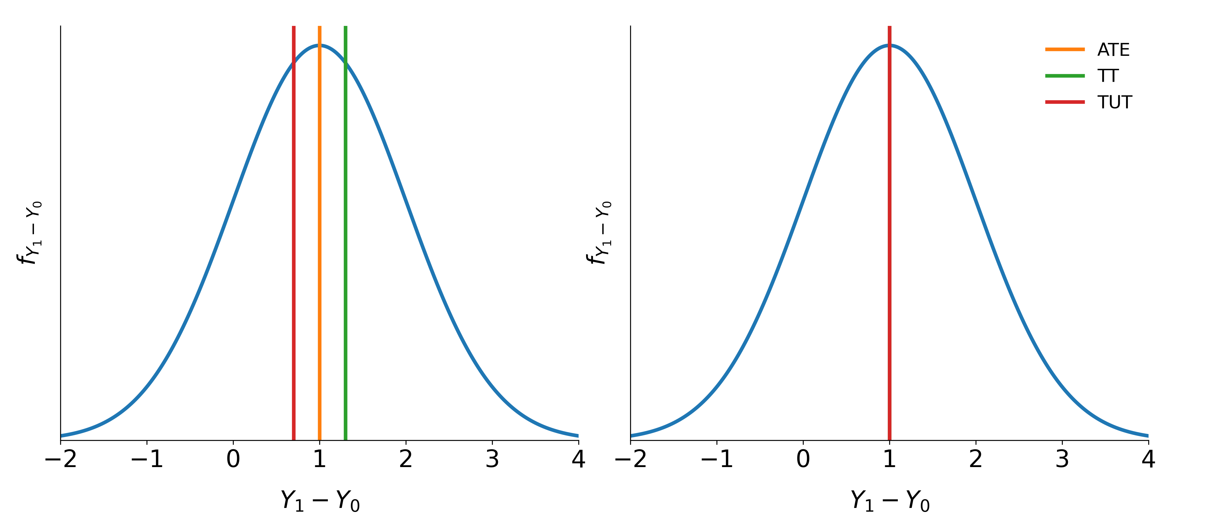
Fig. 1: Conventional treatment effects with and without essential heterogeneity
The policy relevance of the conventional treatment effect parameters is limited in the presence of essential heterogeneity. They are only informative about extreme policy alternatives. The \(B^{ATE}\) is of interest to policy makers if they weigh the possibility of moving a full economy from a baseline to an alternative state or are able to assign agents to treatment at random. The \(B^{TT}\) is informative if the complete elimination of a program already in place is considered. Conversely, if the same program is examined for compulsory participation, then the \(B^{TUT}\) is the policy relevant parameter.
To ensure a tight link between the posed policy question and the parameter of interest, [19] propose the policy-relevant treatment effect \(B^{PRTE}\). They consider policies that do not change potential outcomes, but only affect individual choices. Thus, they account for voluntary program participation.
Policy-Relevant Average Treatment Effect
The \(B^{PRTE}\) captures the average change in outcomes per net person shifted by a change from a baseline state \(B\) to an alternative policy \(A\). Let \(D_B\) and \(D_A\) denote the choice taken under the baseline and the alternative policy regime respectively. Then, observed outcomes are determined as
A policy change induces some agents to change their treatment status \(\left(D_B \neq D_A\right)\), while others are unaffected. More formally, the \(B^{PRTE}\) is then defined as
As an example consider that policy makers want to increase the overall level of education. Rather than directly assigning individuals a certain level of education, policy makers can only indirectly affect schooling choices, e.g. by altering tuition cost through subsidies. The individuals drawn into treatment by such a policy will neither be a random sample of the whole population, nor the whole population of the previously (un-)treated. Therefore the implementation of conventional effects run the risk of being biased, whereas the \(B^{PRTE}\) is able to evaluate the average change in outcomes per net individual that is shifted into treated.
Local Average Treatment Effect
The Local Average Treatment Effect \(B^{LATE}\) was introduced by [26]. They show that instrumental variable approaches (IV) identify \(B^{LATE}\), which measures the mean gross return to treatment for individuals induced into treatment by a change in an instrument.
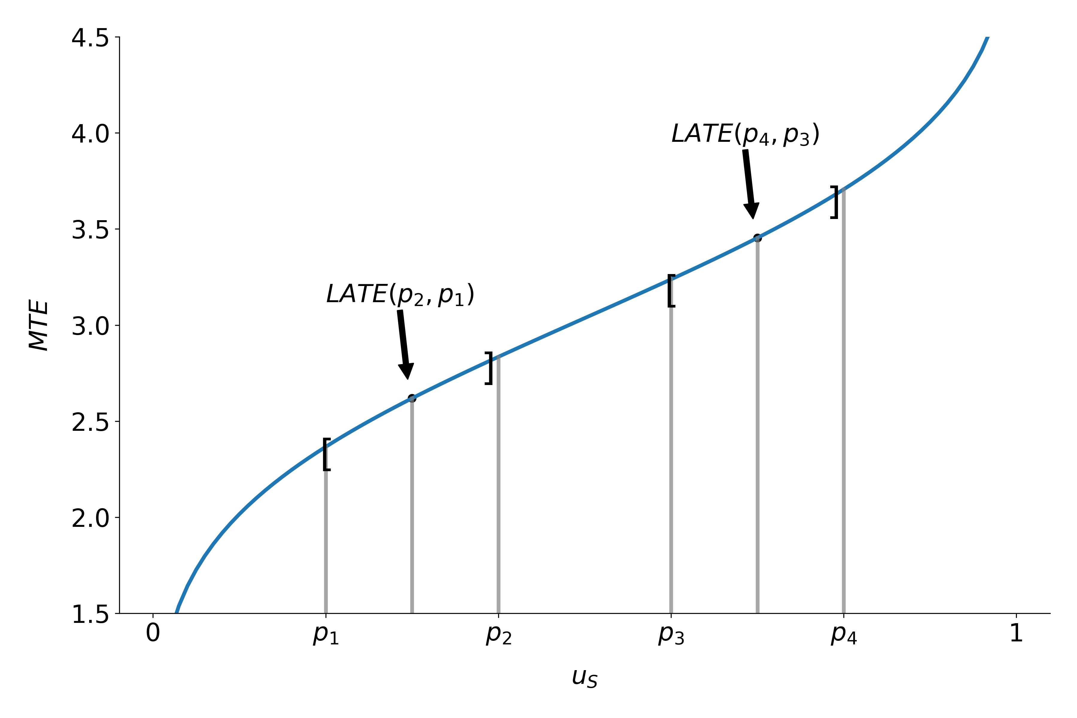
Fig. 2: \(B^{LATE}\) at different values of \(u_S\)
Unfortunately, the people induced to go into treatment by a change in any particular instrument need not to be the same as the people induced to to select into treatment by policy changes other than those corresponding exactly to the variation in the instrument. A desired policy effect may be directly correspond to the variation in the instrument. Moreover, if there is a vector of instruments that generates choice and the components of the vector are intercorrelated, IV estimates using the components of \(Z\) as the instruments, one at a time, do not, in general, identify the policy effect corresponding to varying that instruments, keeping all other instruments fixed, the ceteris paribus effect of the change in the instrument. [14] develop this argument in detail.
The average effect of a policy and the average effect of a treatment are linked by the marginal treatment effect \(\left(B^{MTE}\right)\). The \(B^{MTE}\) was introduced into the literature by [4] and extended by [19], [20] and [21].
Marginal Treatment Effect
The \(B^{MTE}\) is the treatment effect parameter that conditions on the unobserved desire to select into treatment. Let \(V\) be the heterogeneity effect that impacts the propensity for treatment participation and let \(U_S = F_V (V)\). Then, the \(B^{MTE}\) is defined as
The \(B^{MTE}\) is the average benefit for persons with observable characteristics \(X = x\) and unobservables \(U_S = u_S\). By construction, \(U_S\) denotes the different quantiles of \(V\) . So, when varying \(U_S\) but keeping \(X\) fixed, then the \(B^{MTE}\) shows how the average benefit varies along the distribution of \(V\) . For \(U_S\) evaluation points close to zero, the \(B^{MTE}\) is the average effect of treatment for individuals with a value of \(V\) that makes them most likely to participate. The opposite is true for high values of \(U_S\). The \(B^{MTE}\) provides the underlying structure for all average effect parameters previously discussed. These can be derived as weighted averages of the \(B^{MTE}\) ([20]).
Parameter \(j, \Delta j (x)\), can be written as
where the weights \(\omega^{j} (u_S)\) are specific to parameter \(j\), integrate to one, and can be constructed from data. For instance figure 3 shows weights for the \(B^{ATE}\), \(B^{TT}\) and the \(B^{TUT}\) as well as the corresponding \(B^{MTE}\). Contrary, figure 2 emphasizes that the concept of \(B^{LATE}\) is closely related to the idea of \(B^{MTE}\). It illustrates that \(B^{LATE}\) evaluates \(B^{MTE}\) along a particular interval of the distribution of the unobservable Variable \(V\). The specific range depends on the chosen instrument.
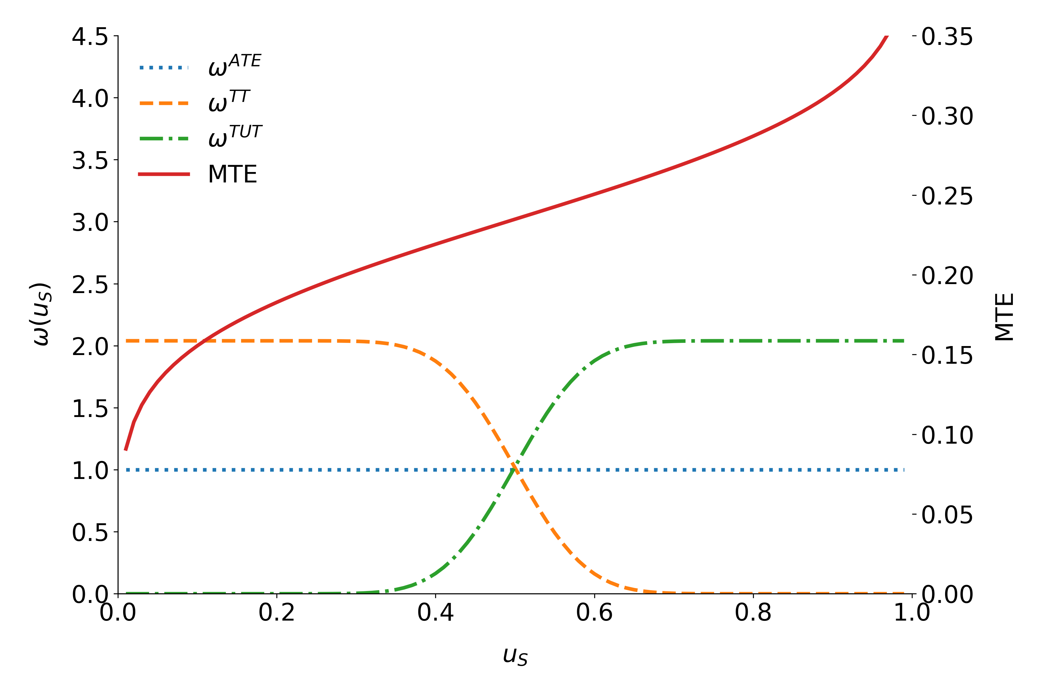
Fig. 3: Weights for the marginal treatment effect for different parameters.
All parameters are identical only in the absence of essential heterogeneity. Then, the \(B^{MTE}(x, u_S)\) is constant across the whole distribution of \(V\) as agents do not select their treatment status based on their unobservable benefits. This can be seen in figure 4 which illustrates \(B^{MTE}\) in the absence of essential heterogeneity, represented by the dotted orange line as well as an example for the \(B^{MTE}\) in the presence of essential heterogeneity portrayed by the blue graph.
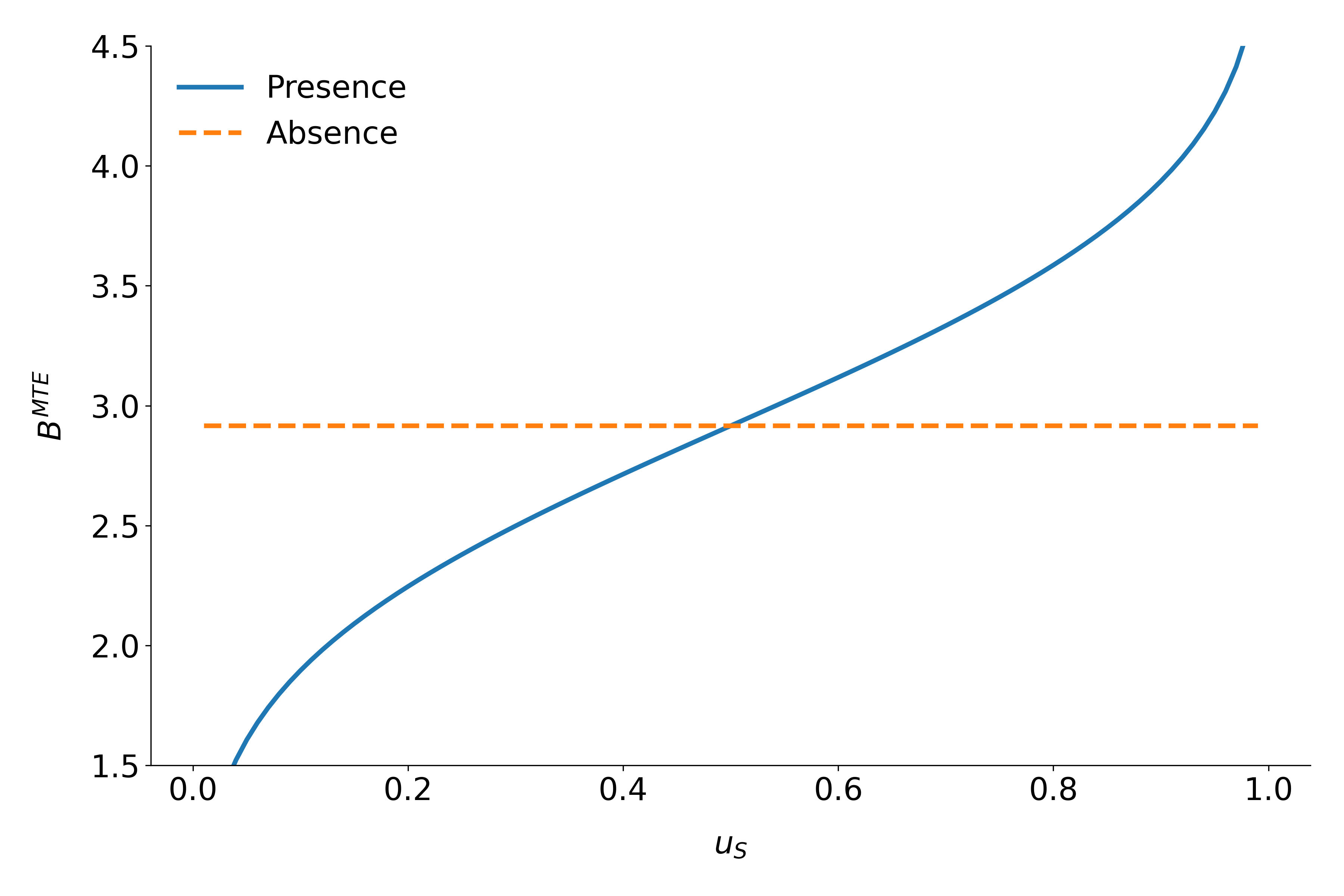
Fig 4: \(B^{MTE}\) in the presence and absence of essential heterogeneity.
So far, we have only discussed average effect parameters. However, these conceal possible treatment effect heterogeneity, which provides important information about a treatment. Hence, we now present their distributional counterparts ([1]).
Distribution of Potential Outcomes
Several interesting aspects of policies cannot be evaluated without knowing the joint distribution of potential outcomes ([2], [17]). The joint distribution of \((Y_1, Y_0)\) allows to calculate the whole distribution of benefits. Based on it, the average treatment and policy effects can be constructed just as the median and all other quantiles. In addition, the portion of people that benefit from treatment can be calculated for the overall population \(Pr(Y_1 - Y_0 > 0)\) or among any subgroup of particular interest to policy makers \(Pr(Y_1 - Y_0 > 0 | X)\). This is important as a treatment which is beneficial for agents on average can still be harmful for some. For a comprehensive overview on related work see [2] and the work they cite. The survey by [12] provides an overview about the alternative approaches to the construction of conterfactual observed outcome distributions. See [3], [31] and [32] for their studies of quantile treatment effects.
The zero of an average effect might be the result of part of the population having a positive effect, which is just offset by a negative effect on the rest of the population. This kind of treatment effect heterogeneity is informative as it provides the starting point for an adaptive research strategy that tries to understand the driving force behind these differences ([24], [25]).
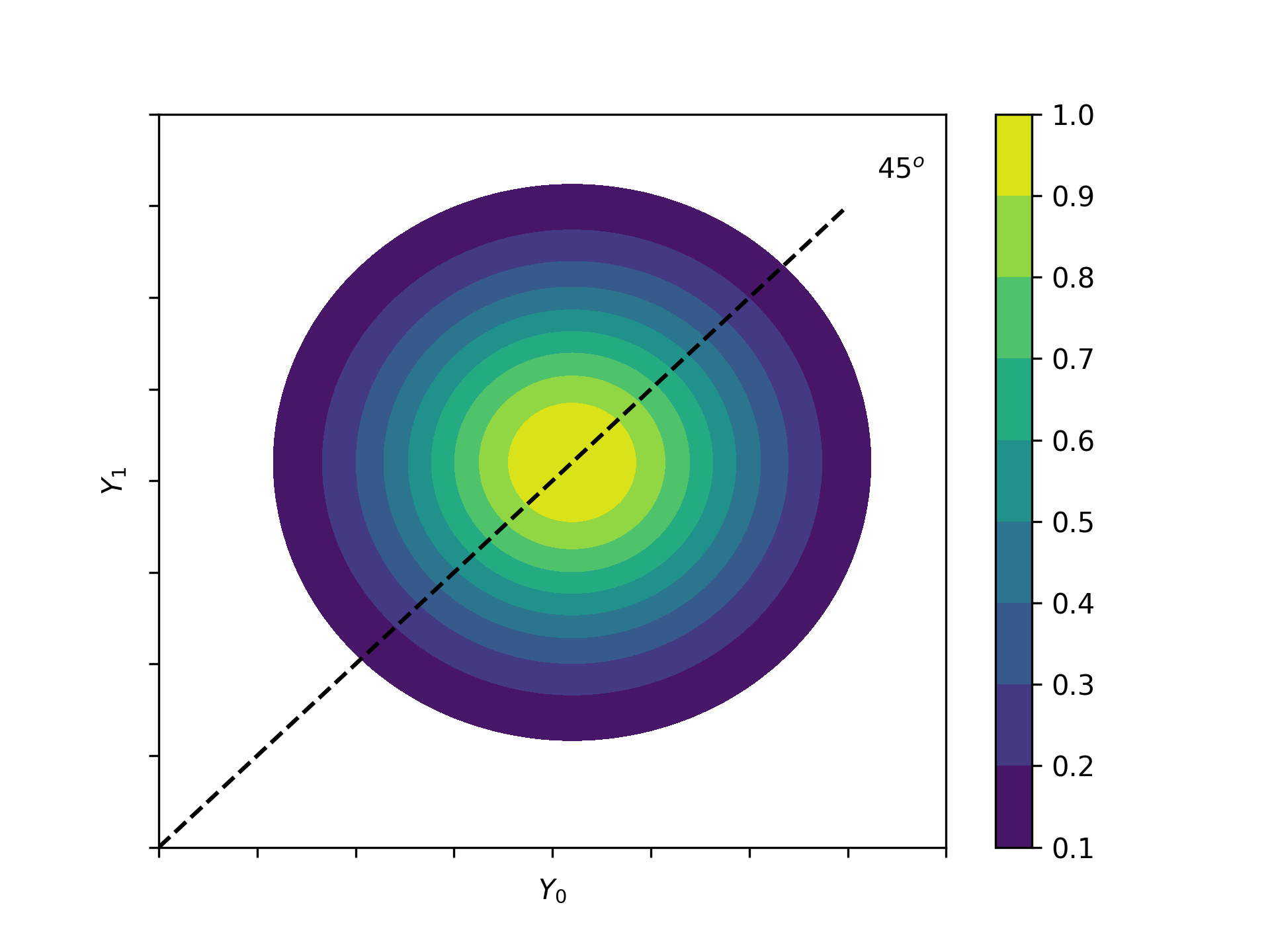
Fig 5: Distribution of potential Outcomes
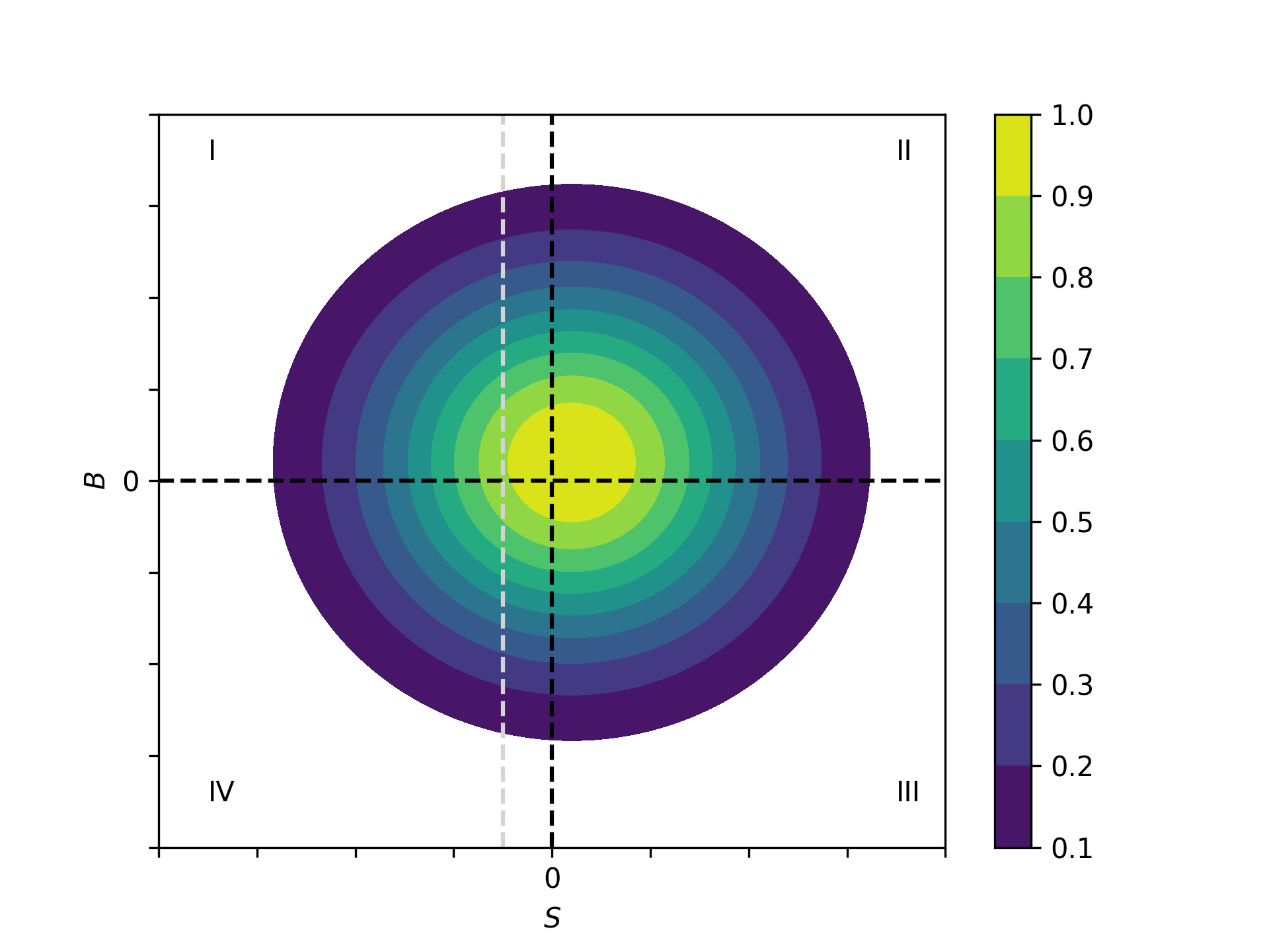
Fig. 6: Distribution of benefits and surplus