Reliability
The following section illustrates the reliability of the estimation strategy behind the grmpy package when facing agent heterogeneity and shows also that the corresponding results withstand a critical examination. The checks in both subsections are based on a mock data set respectively the estimation results from
Carneiro, Pedro, James J. Heckman, and Edward J. Vytlacil. Estimating Marginal Returns to Education. American Economic Review, 101 (6):2754-81, 2011.
We conduct two different test setups. Firstly we show that grmpy is able to provide better results than simple estimation approaches in the presence of essential heterogeneity. For that purpose we rely on a monte carlo simulation setup which enables us to compare the results obtained by the grmpy estimation process with such of a standard Ordinary Least Squares (OLS) approach. Secondly we show that grmpy is capable of replicating the \(B^{MTE}\) results by [6] for the parametric version of the Roy model.
Reliability of Estimation Results
The estimation results and data from [6] build the basis of the reliability test setup. The data is extended by combining them with simulated unobservables that follow a distribution that is pre-specified in the following initialization file. In the next step the potential outcomes and the choice of each individual are calculated by using the estimation results.
This process is iterated a certain amount of times. During each iteration the rate of correlation between the simulated unobservables increases. Translated in the Roy model framework this is equivalent to an increase in the correlation between the unobservable variable \(U_1\) and \(V\), the unobservable that indicates the preference for selecting into treatment. Additionally the specifications of the distributional characteristics are designed so that the expected value of each unobservable is equal to zero. This ensures that the true \(B^{ATE}\) is fixed to a value close to 0.5 independent of the correlation structure.
For illustrating the reliability we estimate \(B^{ATE}\) during each step with two different methods. The first estimation uses a simple OLS approach.
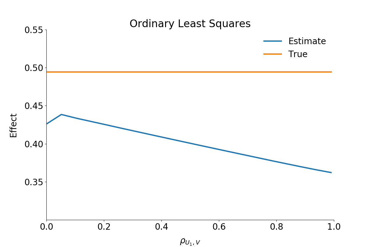
As can be seen from the figure, the OLS estimator underestimates the effect significantly. The stronger the correlation between the unobservable variables the more or less stronger the downwards bias.
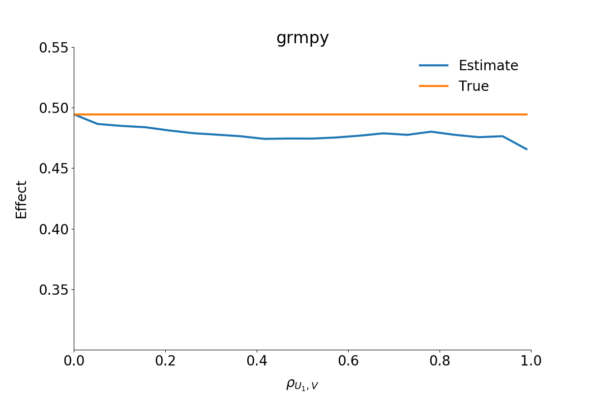
The second figure shows the estimated \(B^{ATE}\) from the grmpy estimation process. Conversely to the OLS results the estimate of the average effect is close to the true value even if the unobservables are almost perfectly correlated.
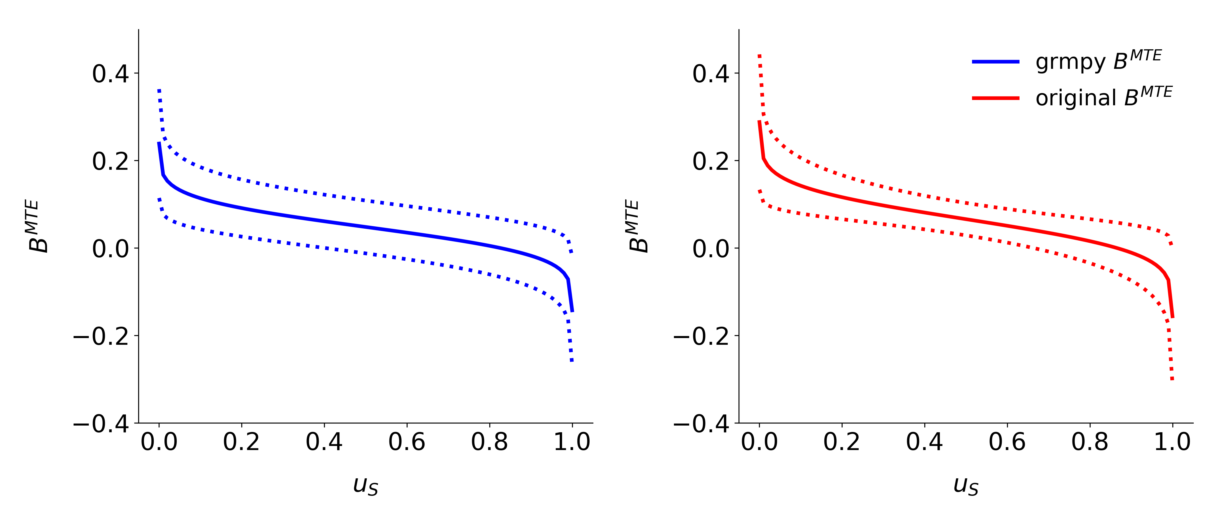
Replication
The second check of reliability compares the results of our estimation process with already existing results from the literature. For this purpose we replicate the results for the marginal treatment effect from Carneiro 2011 ([6]). Additionally we provide a jupyter notebook that runs an estimation based on an initialization file for easy reconstruction of our test setup. The init file corresponds to the specifications of the authors. As shown in the figure below the results are really close to the original results. The deviation seems to be negligible because of the usage of a mock dataset.